Assignment Instructions
- 4 Rectangular CardStock Beams
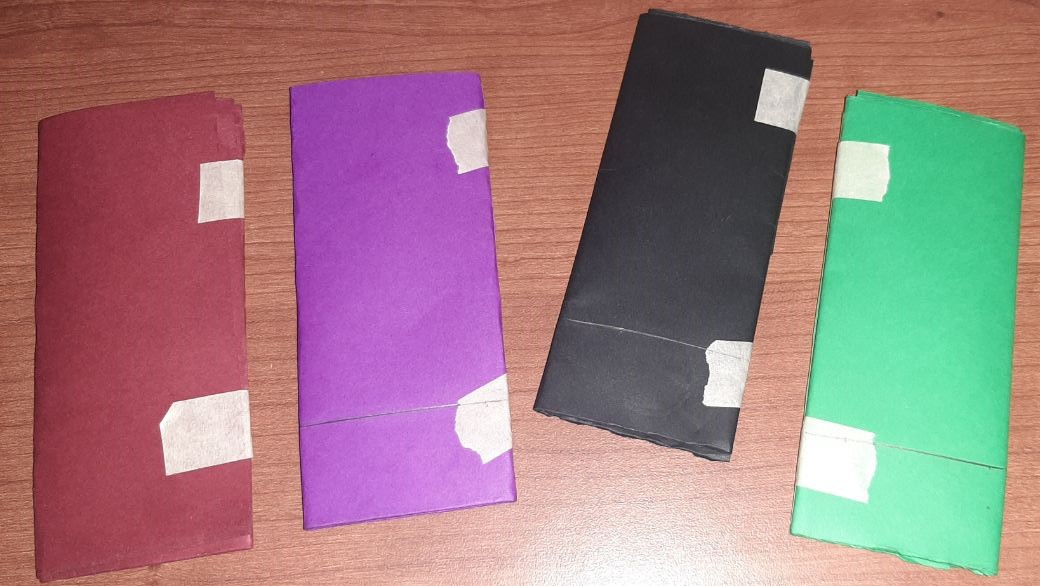
- Table of thickness
| Color | Thickness 1(mm) | Thickness 2(mm) | Average(mm) |
|---|---|---|---|
| Violet | 4.2 | 3.4 | 3.8 |
| Red | 4.4 | 5.3 | 4.85 |
| Green | 4.8 | 3.4 | 4.1 |
| Black | 4.3 | 3.7 | 4.0 |
The beam dimensions used were $50.8mm\times 125mm$. The $50.8mm$ was used because that corresponds to the width dimensions of our sarrus linkages.
3-6. Experiments
5 mass values were used to produce a total of 15 deflection/force results. They ranged from 100 to 500 grams in 100g increments.
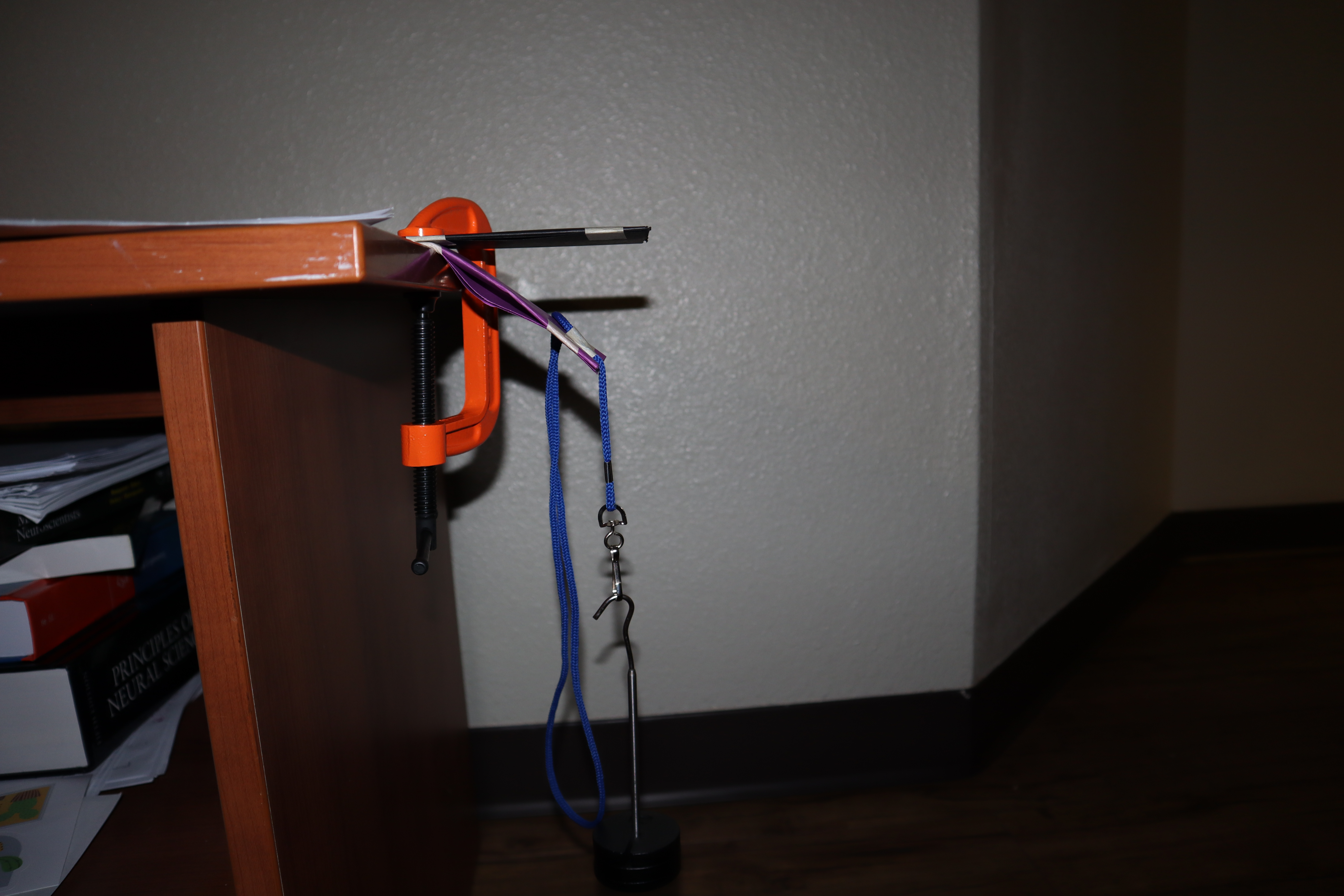
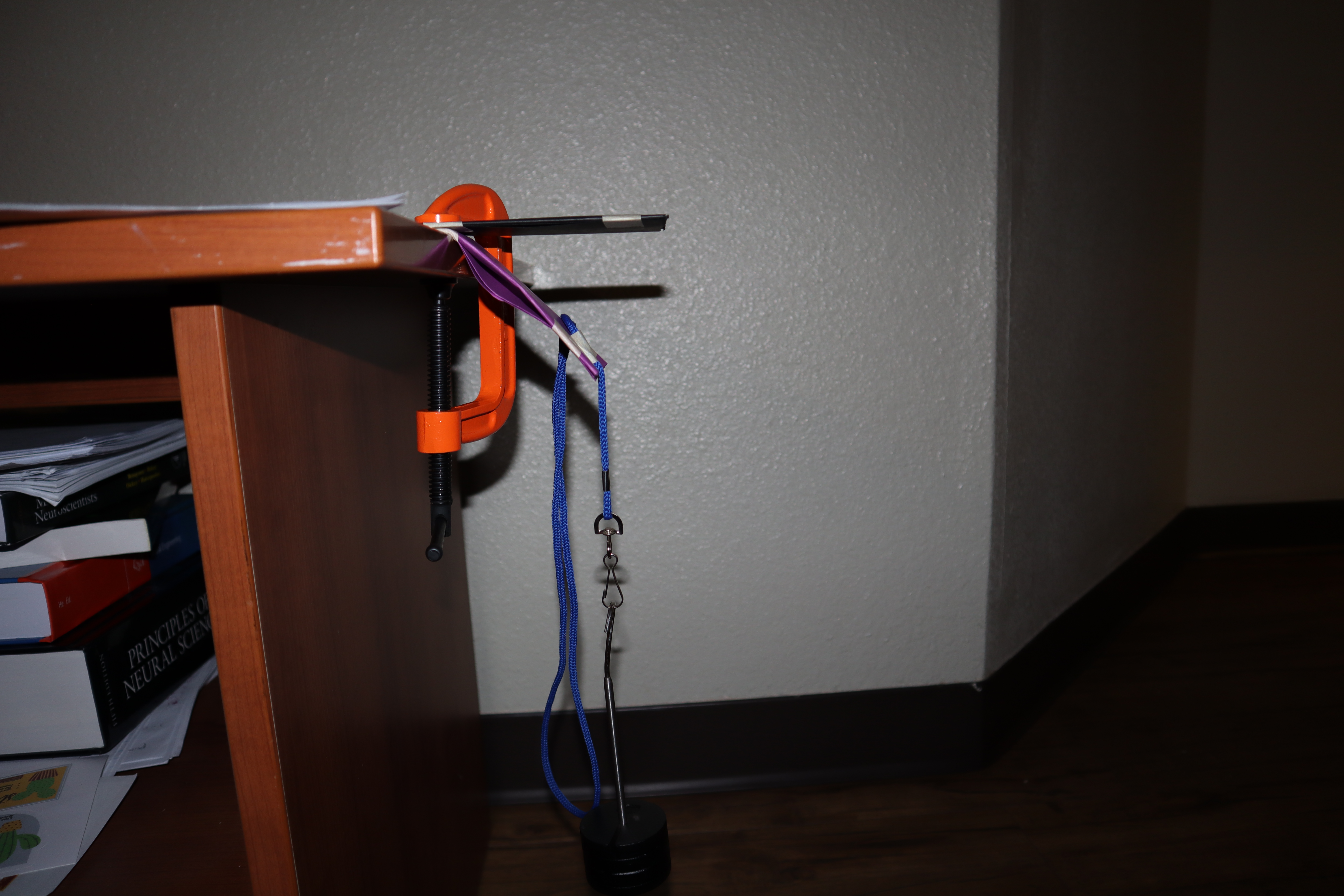
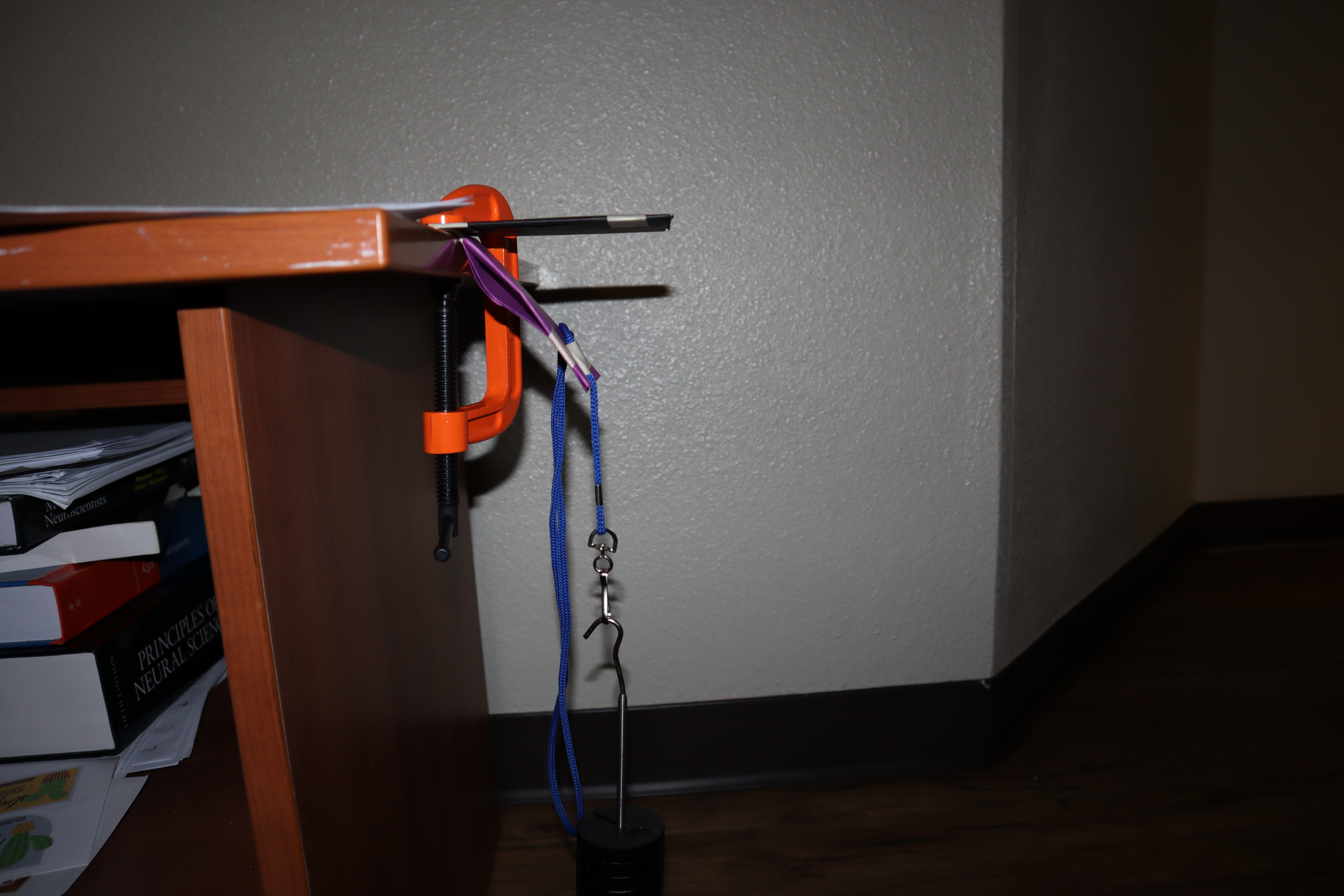
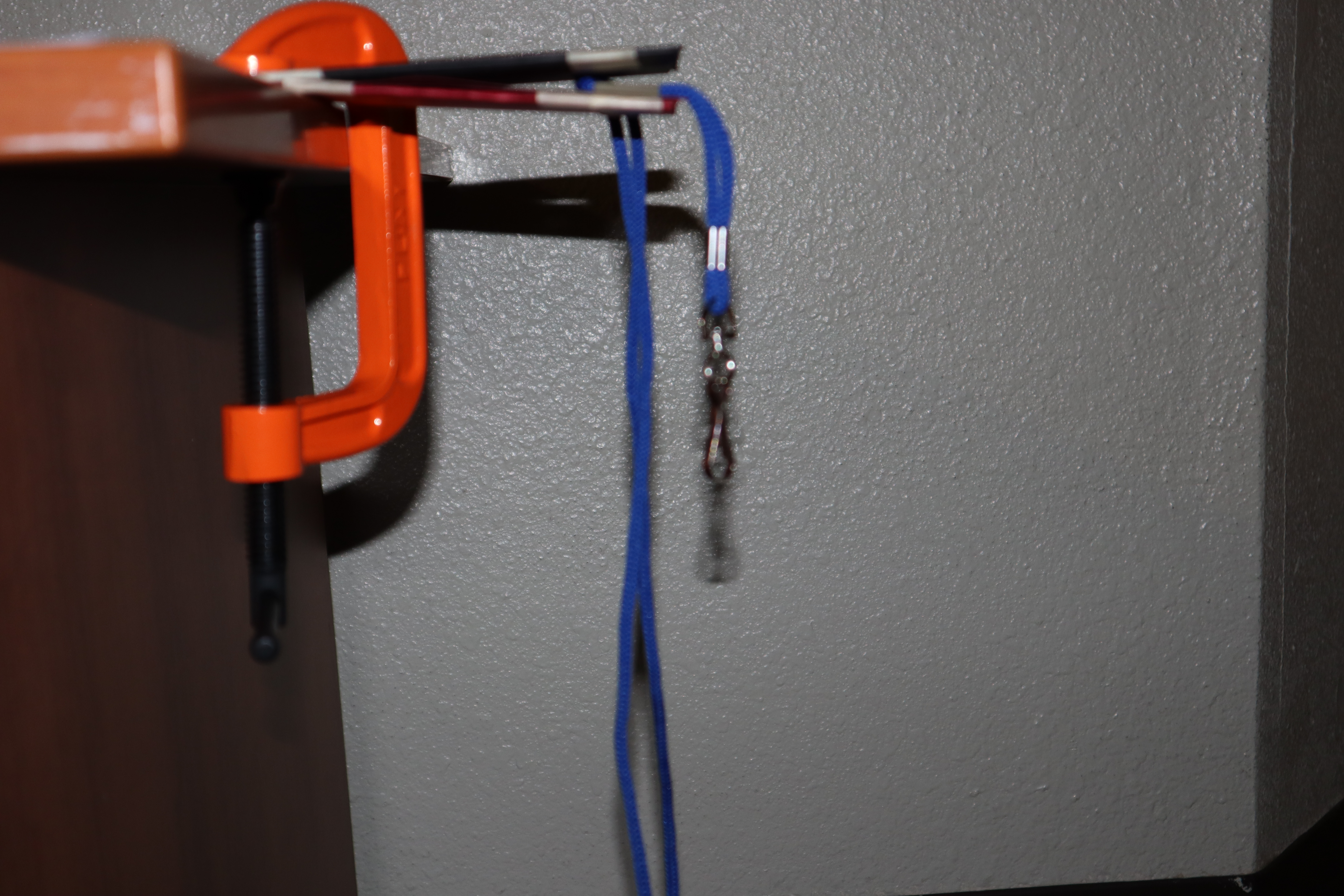
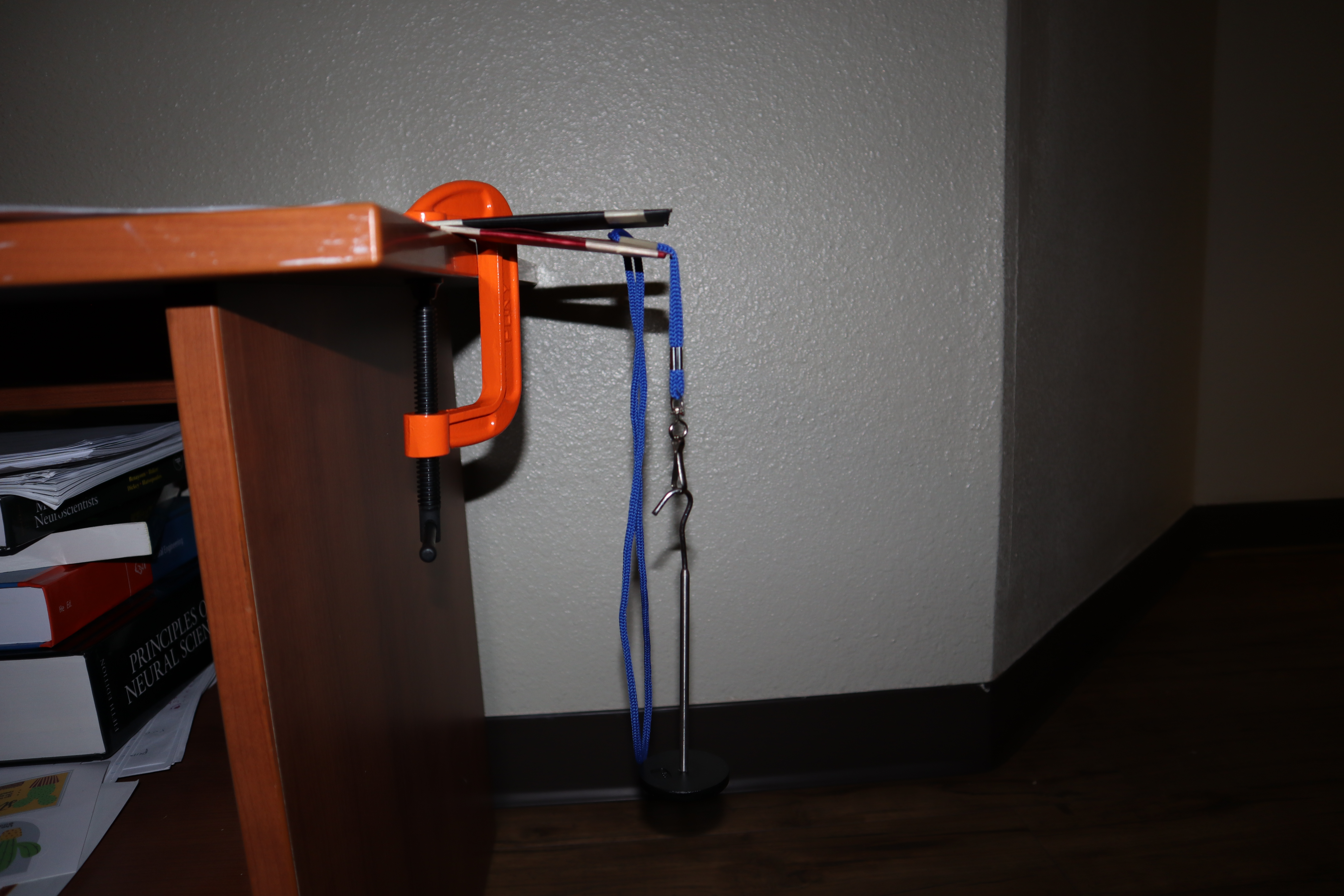
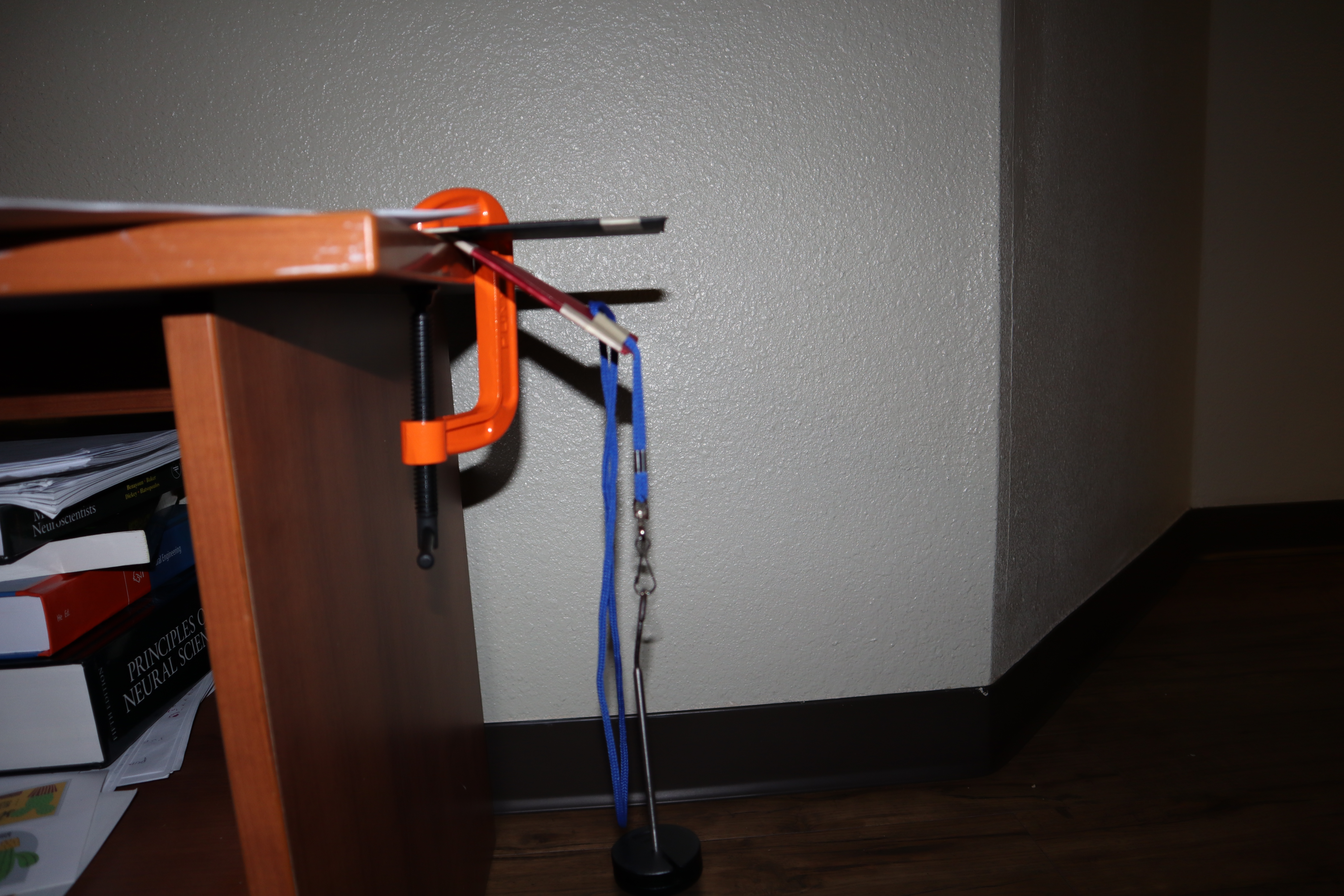
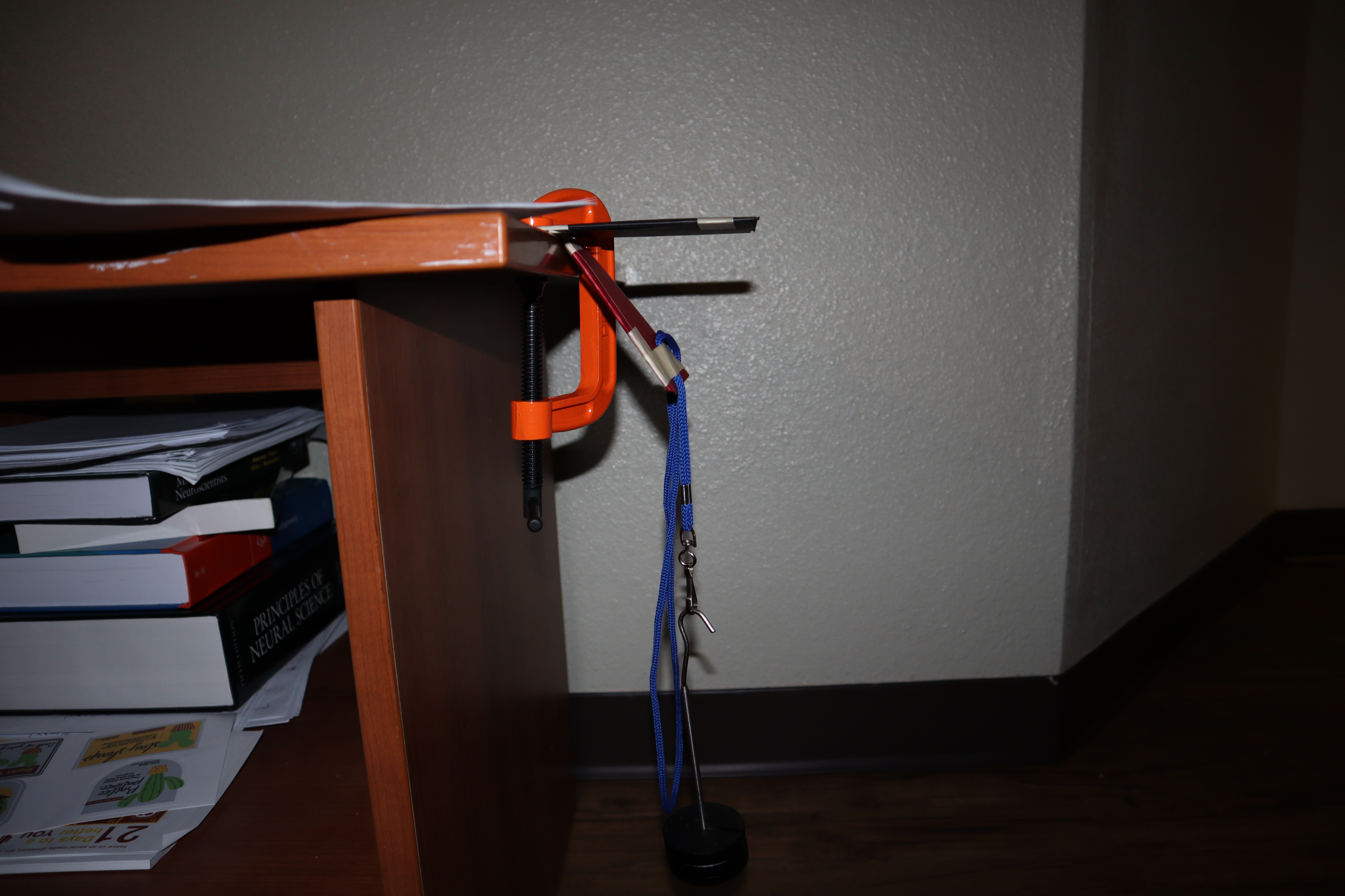
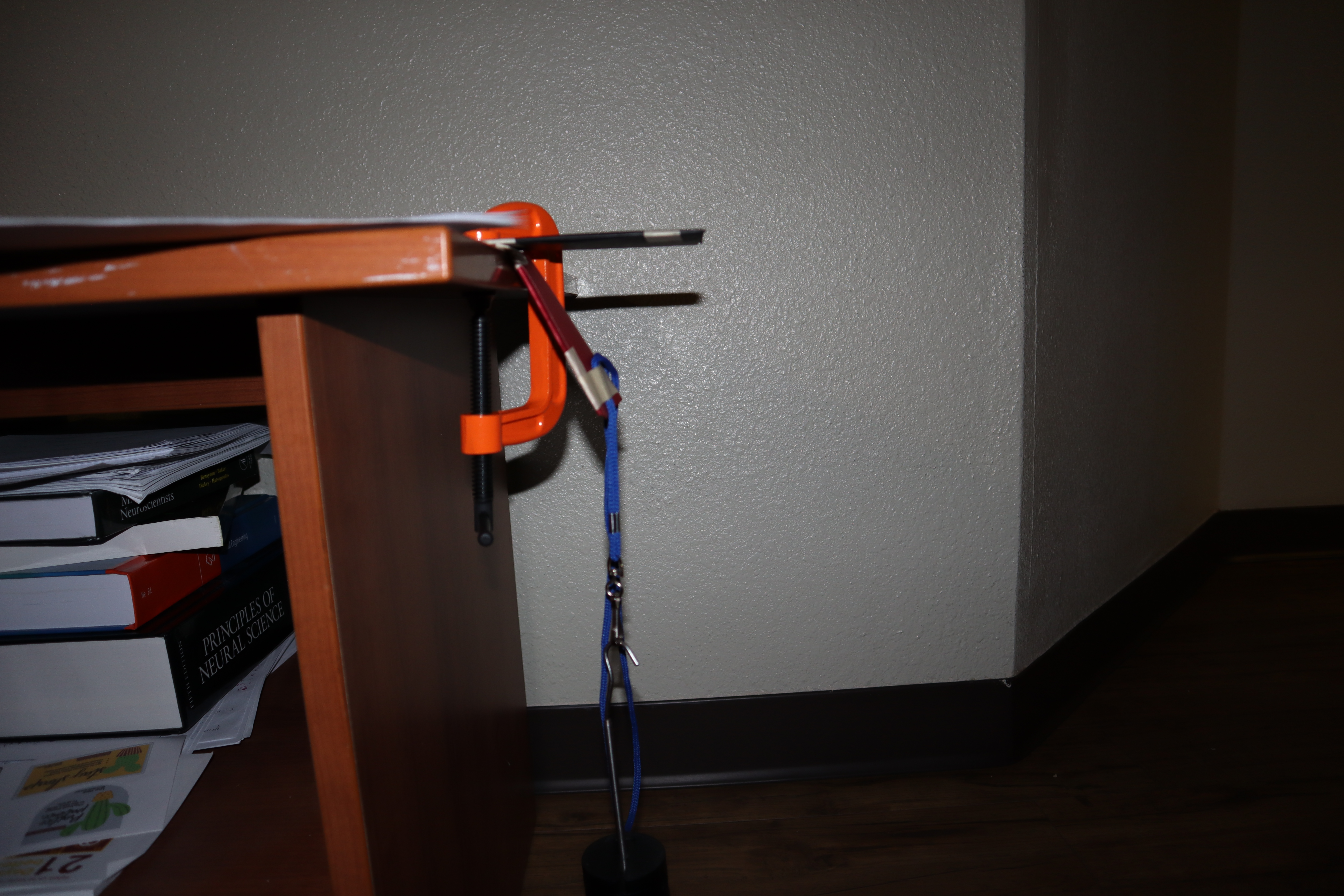
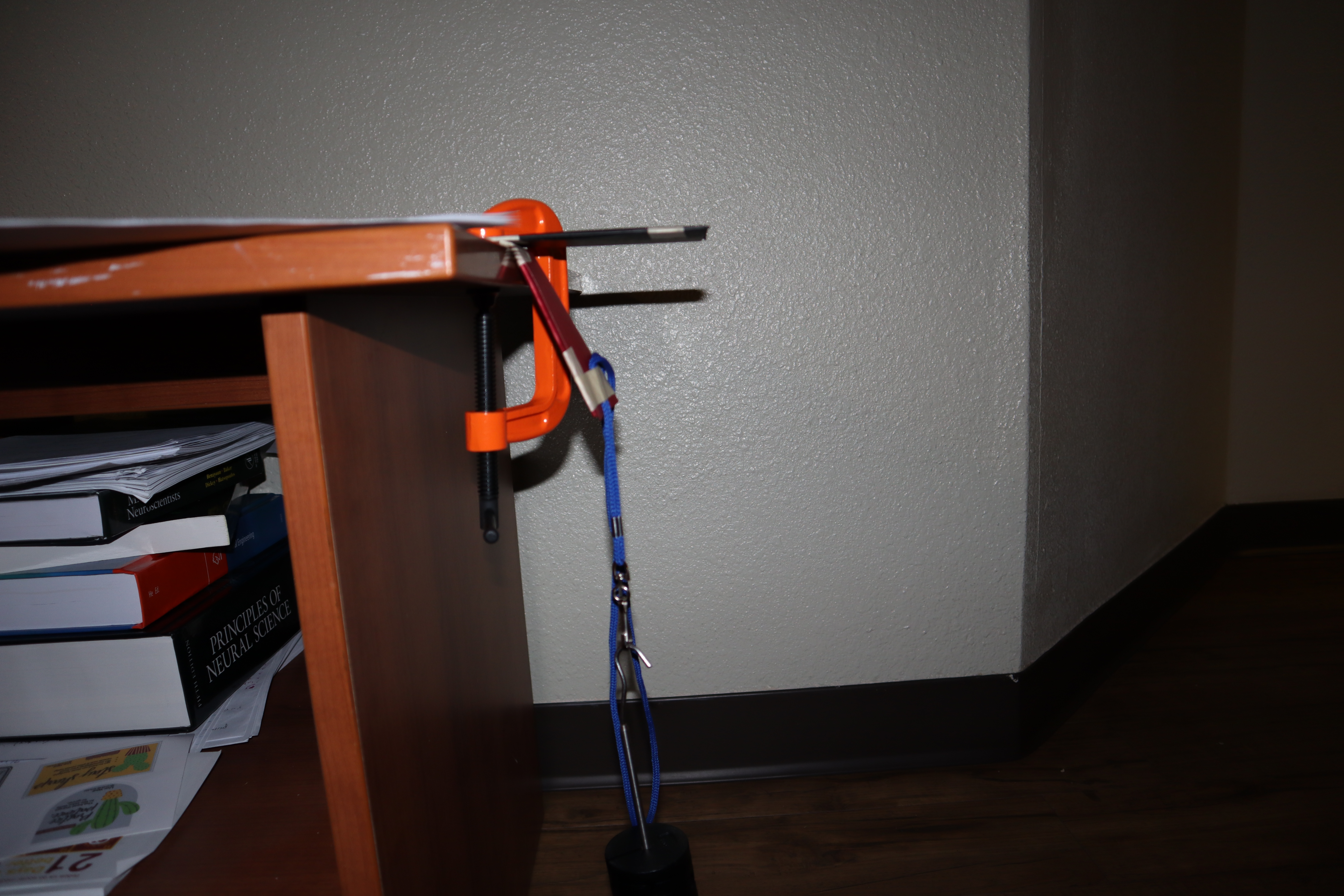
In the experiments, the black beam stayed on top whiles the others were used to produce the recorded values.
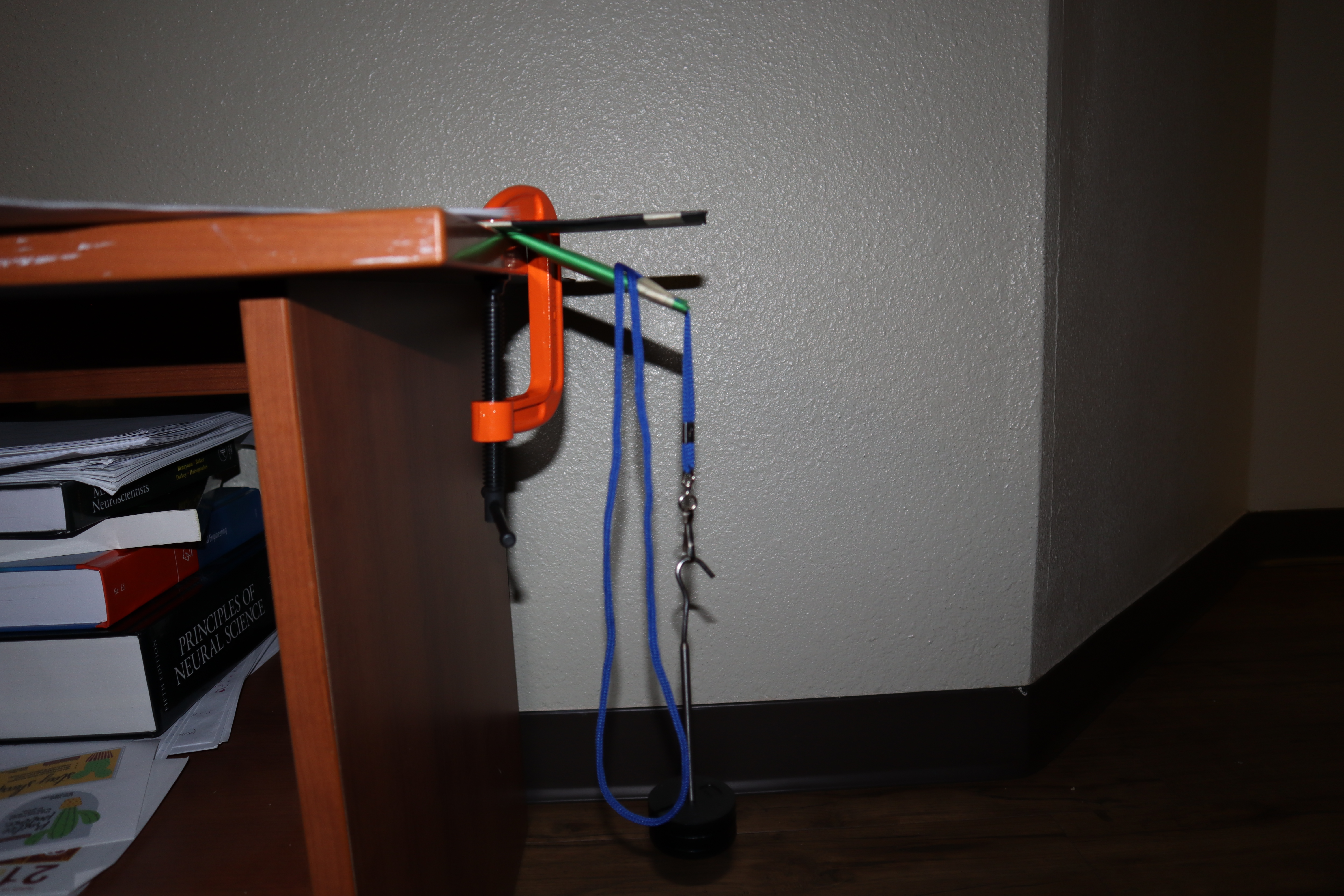
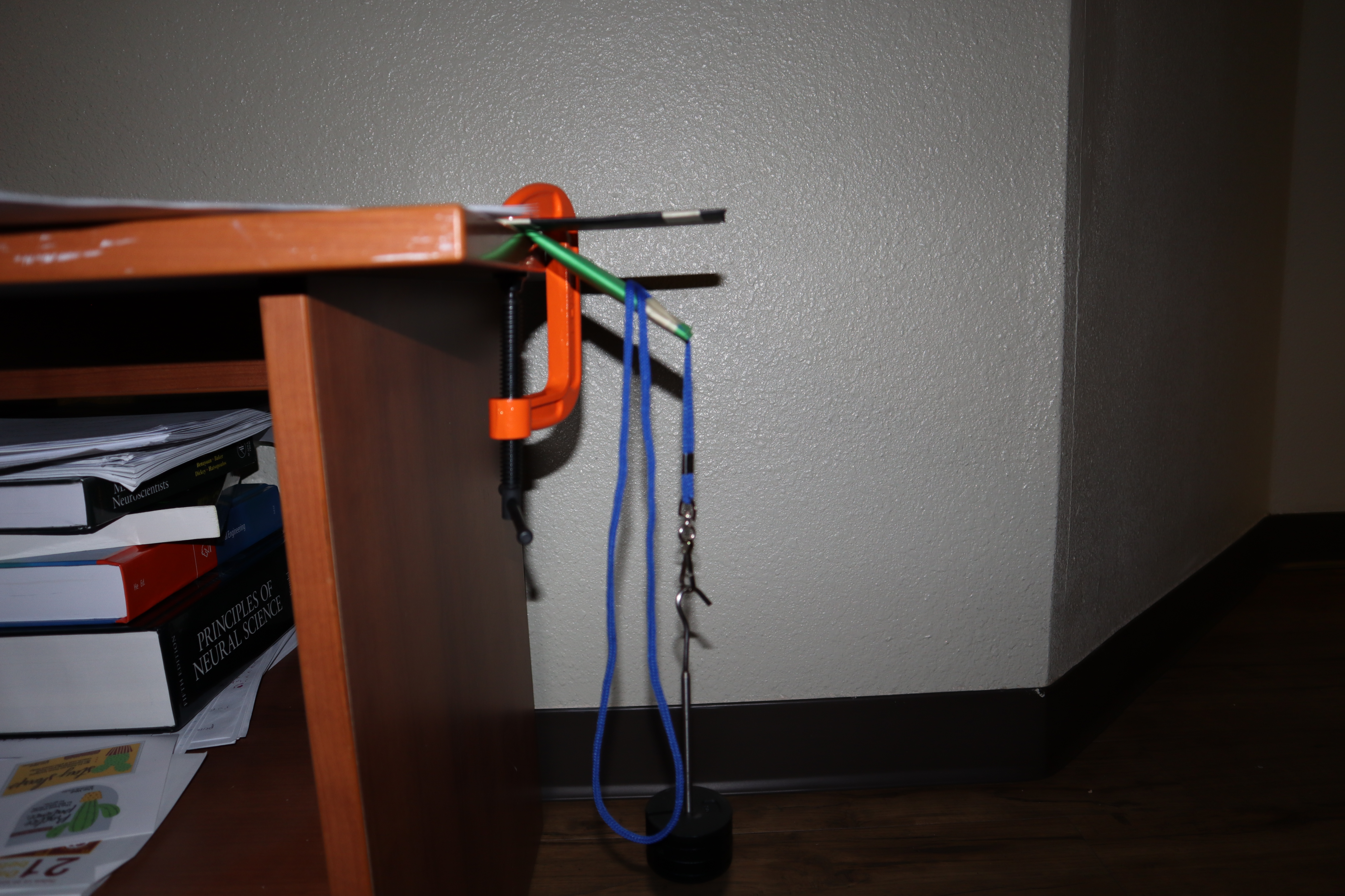
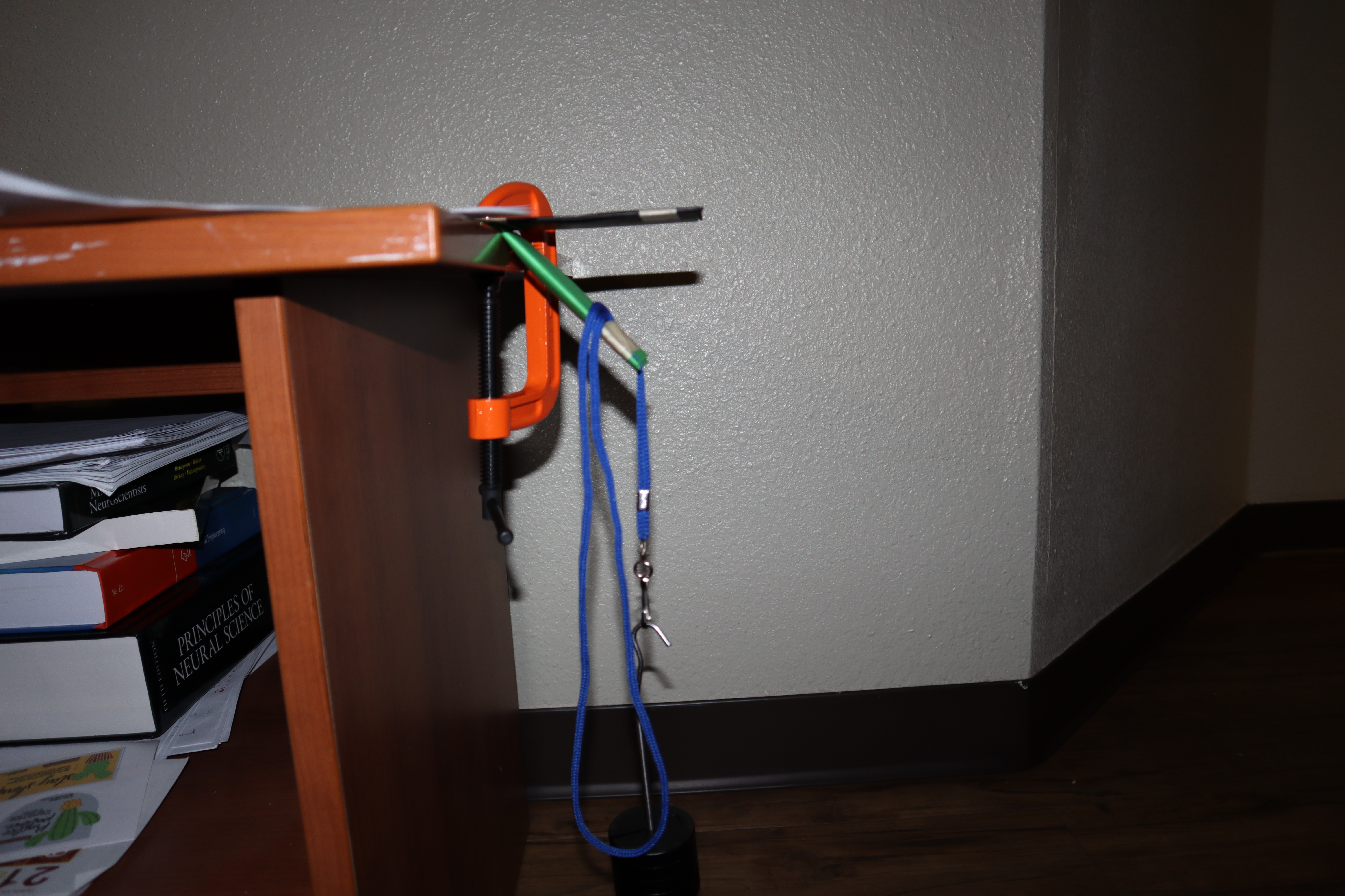
The images below show the different configuration setups used in the experiments.
Violet beam
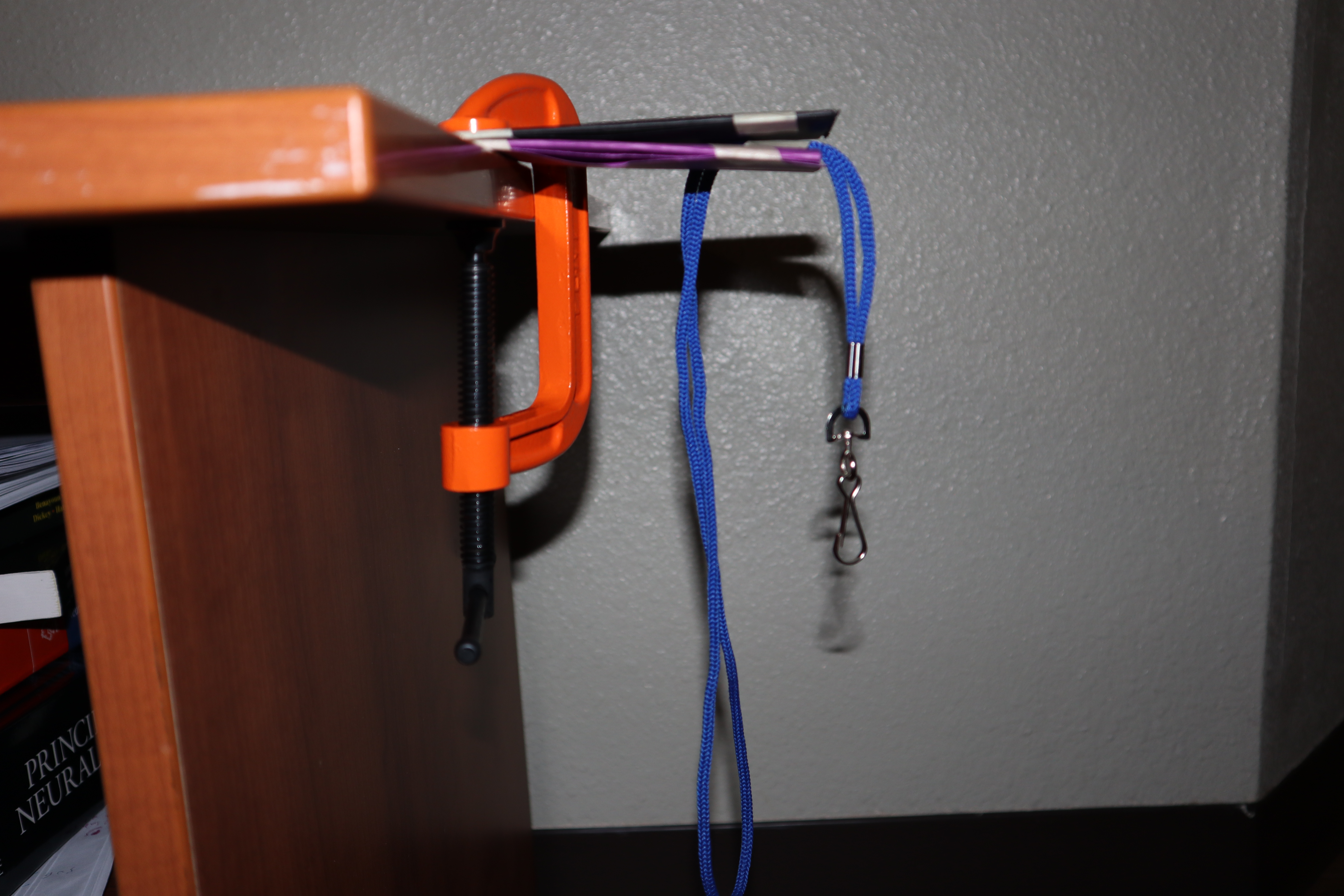
Unloaded
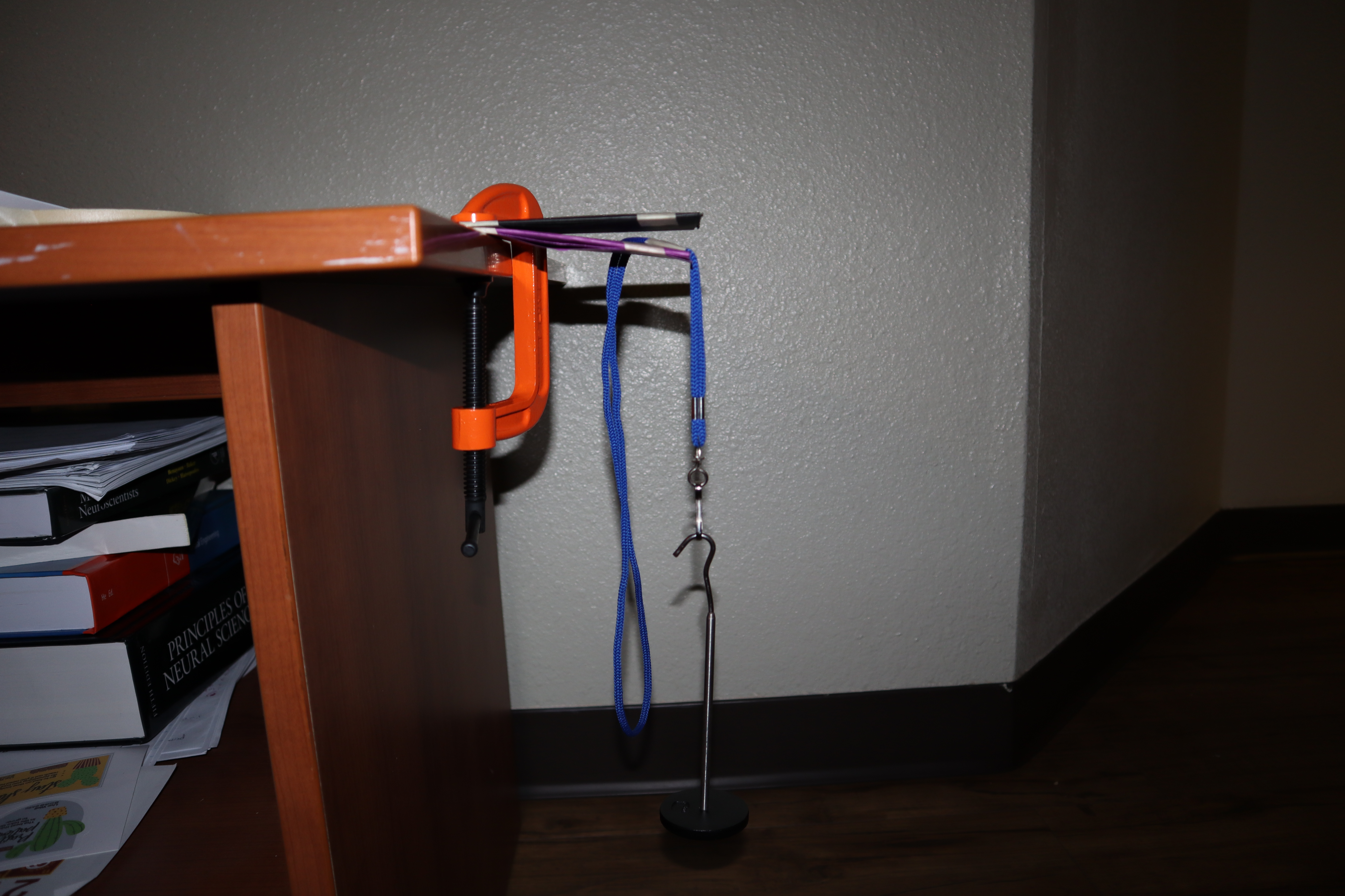
100g
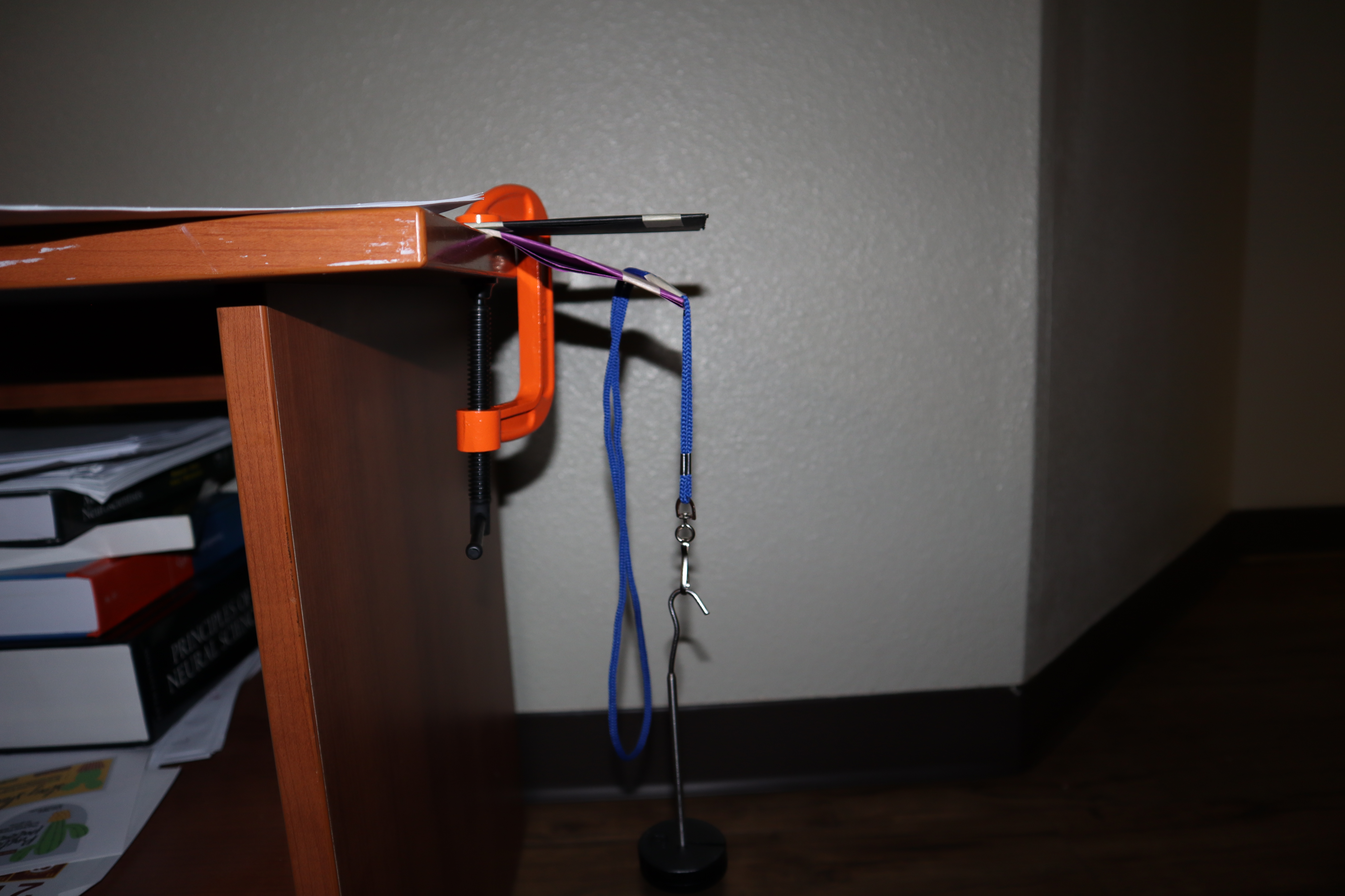
200g
300g
400g
500g
Red beam
Unloaded
100g
200g
300g
400g
500g
Green beam
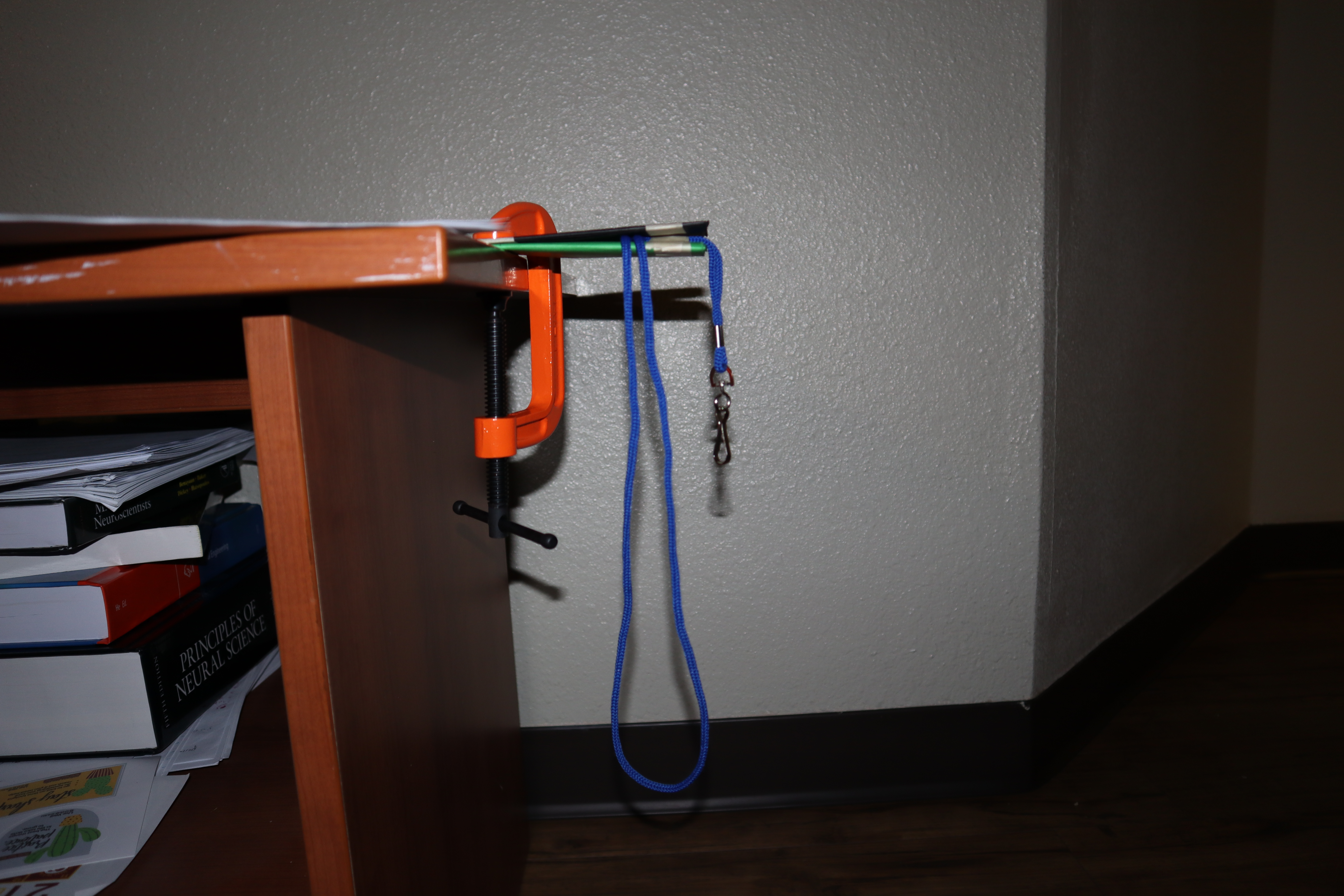
Unloaded
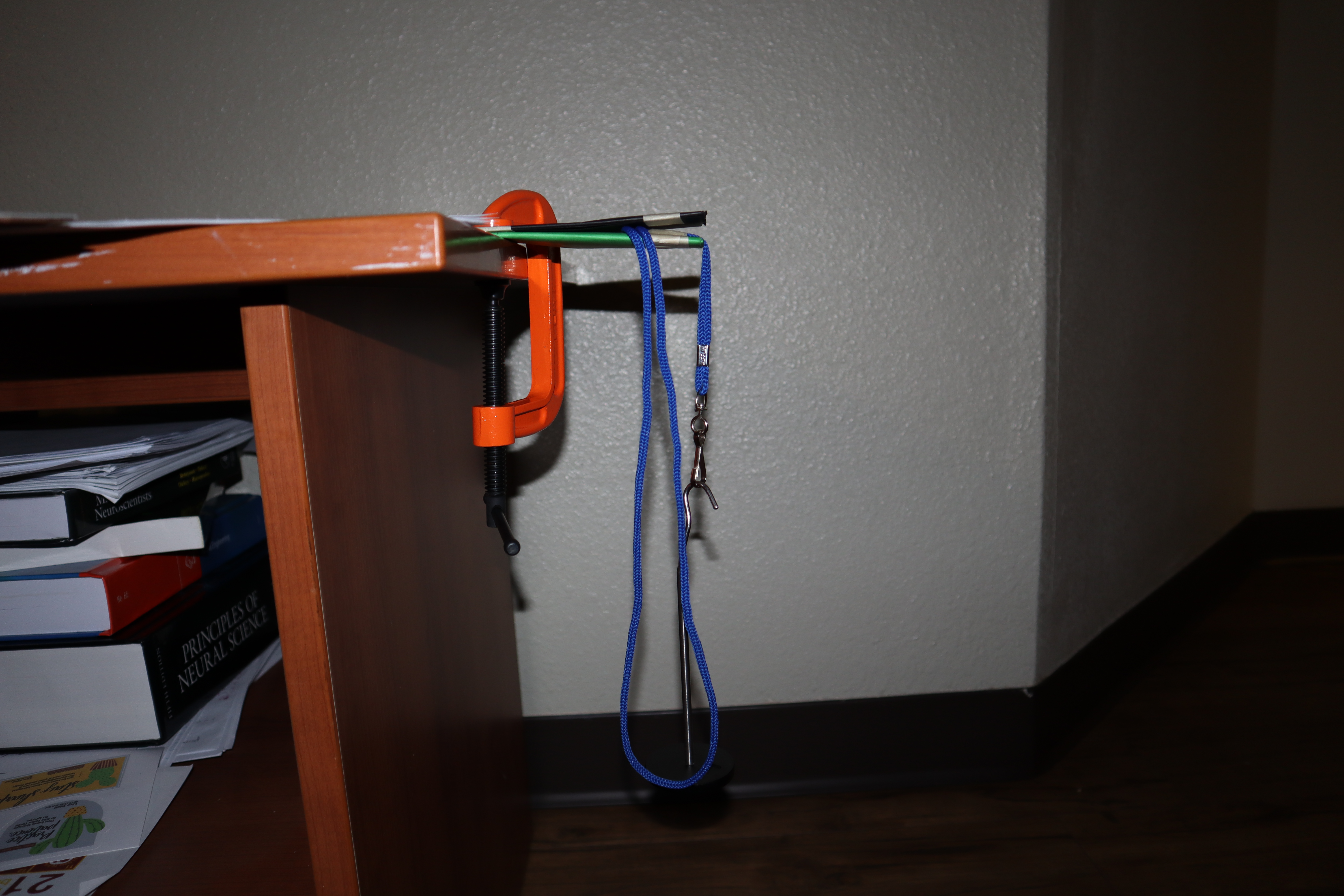
100g
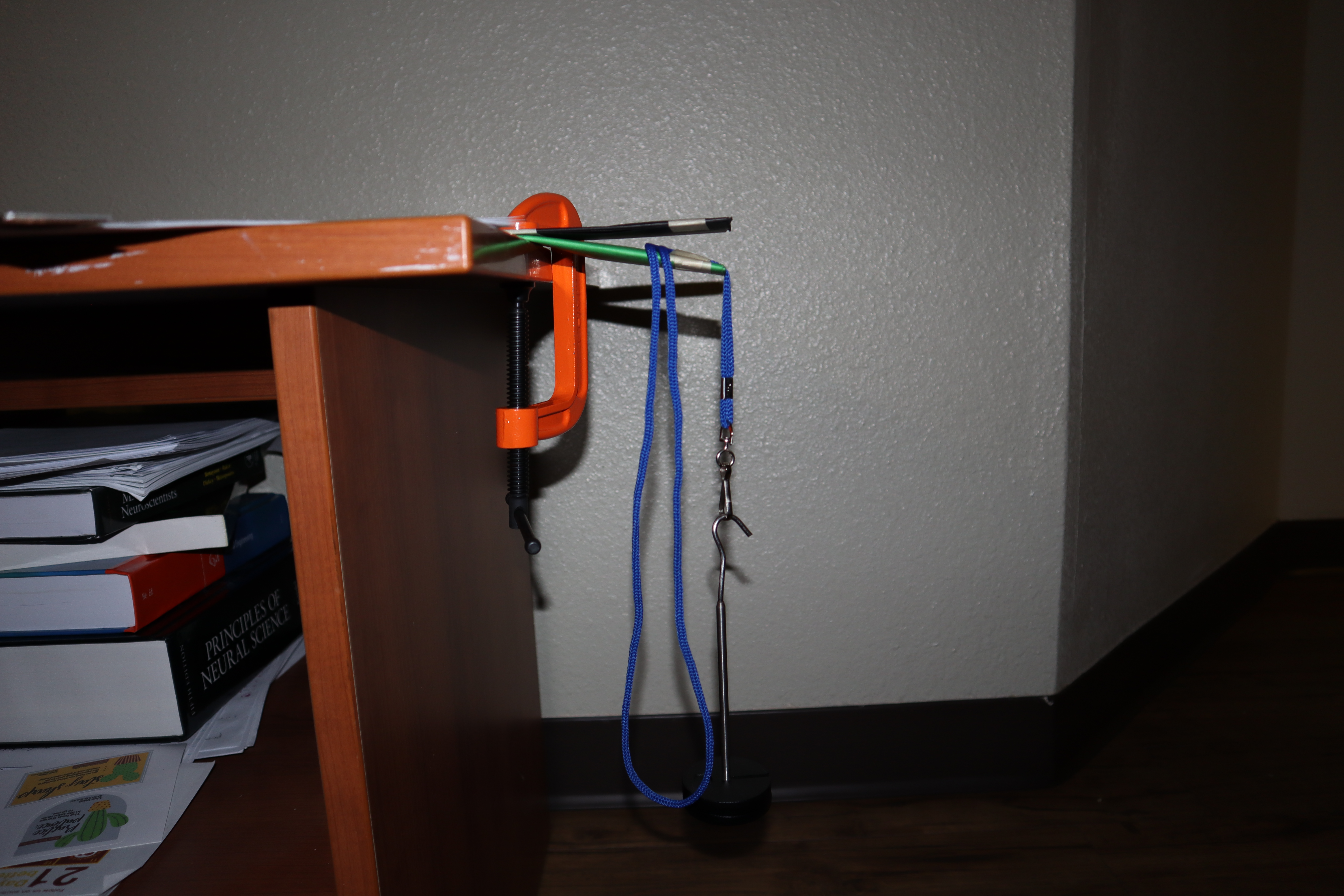
200g
300g
400g
500g
- Table of deflections
| Mass(g) | Deflection_Violet(cm) | Deflection_Red(cm) | Deflection_Green(cm) |
|---|---|---|---|
| 100 | 2.0 | 2.0 | 1.5 |
| 200 | 4.0 | 6.0 | 2.5 |
| 300 | 6.5 | 8.0 | 4.0 |
| 400 | 7.5 | 9.0 | 6.0 |
| 500 | 8.0 | 9.0 | 7.5 |
Plots and Calculations
import numpy as np
import matplotlib.pyplot as plt

masses=list(range(100,600,100))
forces = [9.8*x/1000 for x in masses]
l=0.125 #length
w=0.0508 #width
t=0.0038 #thickness
I=w*(t**3)/12 #Inertia
#violet beam
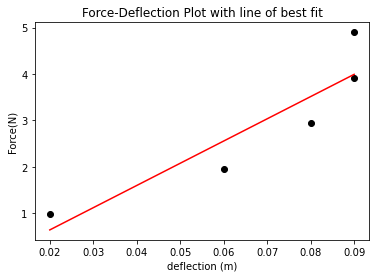
vDeflect = [2,4,6.5,7.5,8.0]
vDeflect = [0.01*x for x in vDeflect]
plt.scatter(vDeflect,forces,color="black")
plt.title("Force-Deflection Plot with line of best fit")
plt.xlabel("deflection (m)")
plt.ylabel("Force(N)")
linear_model=np.polyfit(vDeflect,forces,1)
linear_model_fn=np.poly1d(linear_model)
x_s=np.arange(0,1.5)
plt.plot(vDeflect,linear_model_fn(vDeflect),color="blue")
plt.show()
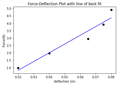
FD=linear_model[0] #slope
E=(FD*(l**3))/(3*I) #Young modulus
E
165653333.11228323
$E = \frac{Pl^3}{3\delta I} =165653333.11228323 Nm^{-2}$
#red beam

rDeflect = [2,6,8,9,9]
rDeflect = [0.01*x for x in rDeflect]

plt.scatter(rDeflect,forces,color="black")
plt.title("Force-Deflection Plot with line of best fit")
plt.xlabel("deflection (m)")
plt.ylabel("Force(N)")

linear_model=np.polyfit(rDeflect,forces,1)
linear_model_fn=np.poly1d(linear_model)

plt.plot(rDeflect,linear_model_fn(rDeflect),color="red")
plt.show()
FD=linear_model[0] #slope
E=(FD*(l**3))/(3*I) #Young modulus
E
134174900.32769114
$E = \frac{Pl^3}{3\delta I} =134174900.32769114 Nm^{-2}$
#green beam

gDeflect = [1.5,2.5,4,6,7.5]
gDeflect = [0.01*x for x in gDeflect]

plt.scatter(gDeflect,forces,color="black")
plt.title("Force-Deflection Plot with line of best fit")
plt.xlabel("deflection (m)")
plt.ylabel("Force(N)")

linear_model=np.polyfit(gDeflect,forces,1)
linear_model_fn=np.poly1d(linear_model)

plt.plot(gDeflect,linear_model_fn(gDeflect),color="green")
plt.show()
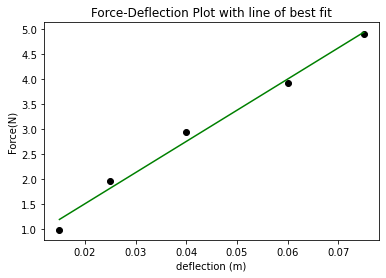
FD=linear_model[0] #slope
E=(FD*(l**3))/(3*I) #Young modulus
E
175197146.5426206
$E = \frac{Pl^3}{3\delta I} = 175197146.5426206 Nm^{-2}$
E_mean = np.mean([175197146.5426206,134174900.32769114,165653333.11228323])
E_mean
158341793.32753167
Using the mean of the 3 values, the yound modulus is approximated as
$E= 158MPa$
The formula for stiffness $k$ is given as \
$k=E\cdot {\frac {A}{L}}$
where
E is the (tensile) elastic modulus (or Young's modulus),
A is the cross-sectional area,
L is the length of the element.
k = E_mean*t*w/l
k
244530.39827157368
$k= 244530Nm^{-1}$